“Deep Learning”: Optimization Techniques

The basic principle used by a number of machine and deep learning algorithms is called supervised learning. You can think of it as learning from mistakes, since it uses iterative procedure to find a minimum of PREDICTION ERROR of a machine learning model for the given training data. The error is usually expressed as a difference between output predicted by the model and actual/target output which is given as a part of training data. This error is calculated using so called LOSS FUNCTION. Mathematical procedure for finding minimum of the error/loss function is known as OPTIMIZATION METHOD. Following this general outline as shown in picture bellow, different machine learning algorithms can be implemented using different models, loss functions and optimization methods. This includes linear regression, logistic regression, feed forward and convolutional neural networks which are explained below.
1. Feature Scaling:

Feature Scaling is a technique to standardize the independent features present in the data in a fixed range. It is performed during the data pre-processing to handle highly varying magnitudes or values or units. If feature scaling is not done, then a machine learning algorithm tends to weigh greater values, higher and consider smaller values as the lower values, regardless of the unit of the values.
Min-Max Normalization: This technique re-scales a feature or observation value with distribution value between 0 and 1.

Standardization: It is a very effective technique which re-scales a feature value so that it has distribution with 0 mean value and variance equals to 1.

Why to scale features
Most of times different features in the data might be have varying magnitudes.For example in a in case of grocery shopping datasets , we usually observe weight of the product in grams or pounds which will be a bigger numbers while price of the product might be dollars which will be lesser numbers.Many of the machine learning algorithms use euclidean distance between data point in their computation.Having two features with different range of numbers will let the feature with bigger range dominate the algorithm.
Where to use Feature Scaling
Before understanding the various methods through which features can be scaled, it is important to understand the importance of feature scaling and the implications if features are not scaled. Many machine learning algorithms require feature scaling as this prevents the model from giving greater weightage to certain attributes as compared to others such as-
Classification models, for example, require features to be scaled as classifiers such as K means use Euclidean distance to calculate the distance between two points and if one feature is in different units of measurement causing it to have a broad range of values then it can influence the calculation causing biased and wrong results. Thus the change in the metric space i.e. the Euclidean distance between two samples will be different after transformation.
Gradient descent which is an optimization algorithm often used in Logistic Regression, SVM, Neural Networks etc. is another prominent example where if features are on different scale, certain weights are updated faster than others. However, feature scaling helps in causing Gradient Descent to converge much faster as standardizing all the variables on to the same scale, for example, for a linear regression makes it easy to calculate the slope ( y = mx + c) (where we normalize the M parameter to converge faster).
Feature Extraction techniques such as Principal Component Analysis (PCA), Kernel Principal Component Analysis (Kernel PCA), Linear discriminant analysis (LDA) where we have to find directions by maximizing the variance, by scaling the features we can avoid a potential error of emphasizing variables that have large scales of measurement. For example, if we have one component (e.g. work duration per day) where variation is less than another (e.g. monthly income) because of their respective scales (hours vs. dollars), PCA might determine that the direction of maximal variance corresponds more closely with the ‘income’ axis. If the features are not scaled, a change in income of one dollar can be considered much more important than a change in the duration of one hour. Generally, the only family of algorithms that can be called scale-invariant are tree-based methods otherwise all the other algorithms such as the Neural Networks tend to converge faster, K-Means generally gives better clustering results and various Feature Extraction process provide better outcomes with pre-processed scaled features.
Advantages :
This method is used when algorithms such as k-nearest neighbour where distances are to be calculated or regression where coefficients are to be prepared. In models where the functioning of the model relies on the magnitude of values, normalization is often done. However, for all the above-mentioned scenarios, standardization (mentioned below) is more commonly used. There are certain applications where min-max scaling is more useful than standardization such as in models where image processing is required. For example in various classification models where images are classified based on the pixel intensities which range between 0 to 255 (for RGB colour range i.e. for coloured images), the rescaling process requires the values to be normalized within this range only. Various Neural Network algorithms also require the values of features to range between 0 and 1 and Min-Max scaling comes in handy here.
disadvantages :
Feature scaling usually helps, but it is not guaranteed to improve performance. If you use distance-based methods like SVM, omitting scaling will basically result in models that are disproportionately influenced by the subset of features on a large scale. It may well be the case that those features are in fact the best ones you have. In that case, scaling will reduce performance.
2. Batch normalization :

Why do we use batch normalization?
We normalize the input layer by adjusting and scaling the activations. For example, when we have features from 0 to 1 and some from 1 to 1000, we should normalize them to speed up learning. If the input layer is benefiting from it, why not do the same thing also for the values in the hidden layers, that are changing all the time, and get 10 times or more improvement in the training speed.
Batch normalization reduces the amount by what the hidden unit values shift around (covariance shift). To explain covariance shift, let’s have a deep network on cat detection. We train our data on only black cats’ images. So, if we now try to apply this network to data with colored cats, it is obvious; we’re not going to do well. The training set and the prediction set are both cats’ images but they differ a little bit. In other words, if an algorithm learned some X to Y mapping, and if the distribution of X changes, then we might need to retrain the learning algorithm by trying to align the distribution of X with the distribution of Y.
How does batch normalization work?
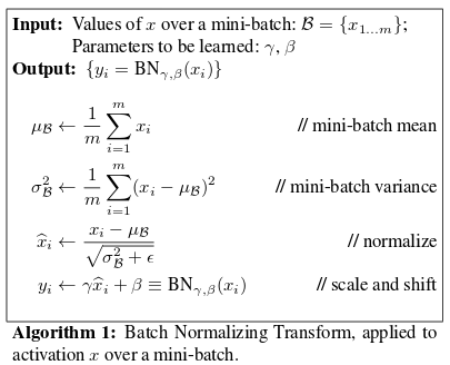
To increase the stability of a neural network, batch normalization normalizes the output of a previous activation layer by subtracting the batch mean and dividing by the batch standard deviation.
However, after this shift/scale of activation outputs by some randomly initialized parameters, the weights in the next layer are no longer optimal. SGD ( Stochastic gradient descent) undoes this normalization if it’s a way for it to minimize the loss function.
Consequently, batch normalization adds two trainable parameters to each layer, so the normalized output is multiplied by a “standard deviation” parameter (gamma) and add a “mean” parameter (beta). In other words, batch normalization lets SGD do the denormalization by changing only these two weights for each activation, instead of losing the stability of the network by changing all the weights.
Advantages :
- Reduces the vanishing gradients problem
- Less sensitive to the weight initialization
- Able to use much larger learning rates to speed up the learning process
- Acts like a regularize
disadvantages :
- Slower predictions due to the extra computations at each layer
3. Mini Batch Gradient descent (MGD) :

Mini-batch gradient descent is a variation of the gradient descent algorithm that splits the training datasets into small batches that are used to calculate model error and update model coefficients.
Let us understand like this,
suppose I have 1000 records and my batch size = 50, I will choose randomly 50 records, then calculate summation of loss and then send the loss to optimizer to find dE/dw.
What is batch size?
The batch size defines the number of samples that will be propagated through the network.
For instance, let’s say you have 1050 training samples and you want to set up a batch_size equal to 100. The algorithm takes the first 100 samples (from 1st to 100th) from the training dataset and trains the network. Next, it takes the second 100 samples (from 101st to 200th) and trains the network again. We can keep doing this procedure until we have propagated all samples through of the network. Problem might happen with the last set of samples. In our example, we’ve used 1050 which is not divisible by 100 without remainder. The simplest solution is just to get the final 50 samples and train the network.
Advantages :
- The model update frequency is higher than BGD: In MGD, we are not waiting for entire data, we are just passing 50 records or 200 or 100 or 256, then we are passing for optimization.
- The batching allows both efficiency of not having all training data in memory and algorithms implementations. We are controlling memory consumption as well to store losses for each and every datasets.
- The batches updates provide a computationally more efficient process than SGD.
disadvantages :
- No guarantee of convergence of a error in a better way.
- Since the 50 sample records we take , are not representing the properties (or variance) of entire datasets. Do, this is the reason that we will not be able to get an convergence i.e., we won’t get absolute global or local minima at any point of a time.
- While using MGD, since we are taking records in batches, so, it might happen that in some batches, we get some error and in dome other batches, we get some other error. So, we will have to control the learning rate by ourself , whenever we use MGD. If learning rate is very low, so the convergence rate will also fall. If learning rate is too high, we won’t get an absolute global or local minima. So we need to control the learning rate.
4. Gradient descent with momentum :

Gradient descent with momentum will always work much faster than the algorithm Standard Gradient Descent. The basic idea of Gradient Descent with momentum is to calculate the exponentially weighted average of your gradients and then use that gradient instead to update your weights.It functions faster than the regular algorithm for the gradient descent.
How it works ?
Consider an example where we are trying to optimize a cost function that has contours like the one below and the red dot denotes the local optima (minimum) location.

We start gradient descent from point ‘A’ and we through end up at point ‘B’ after one iteration of gradient descent, the other side of the ellipse. Then another phase of downward gradient can end at ‘C’ level. With through iteration of gradient descent, with oscillations up and down, we step towards the local optima. If we use higher learning rate then the frequency of the vertical oscillation would be greater.This vertical oscillation therefore slows our gradient descent and prevents us from using a much higher learning rate.
By using the exponentially weighted average dW and db values, we tend to average the oscillations in the vertical direction closer to zero as they are in both (positive and negative) directions. Whereas all the derivatives point to the right of the horizontal direction in the horizontal direction, the average in the horizontal direction will still be quite large. It enables our algorithm to take a straighter forward path to local optima and to damp out vertical oscillations. Because of this the algorithm will end up with a few iterations at local optima.

Implementation :

Advantages :
The above issue led to the birth of momentum based gradient descent update rule, where, ‘w’ and ‘b’ are updated not just based on the current updates(derivative), but also the past updates(derivatives). ‘gamma * vt-1’ represents the history component.
With the history component, during every timestep, the gradient moves the current direction as well as the previous gradient direction, where ‘gamma’ value ranges from 0 to 1. Hence momentum based gradient descent update rule takes the exponentially decaying averages of the gradient.
Disadvantages :
Momentum-based GD is able to take larger steps even in the regions of the gentle slopes, as the momentum of the history gradients is carried with it every step. But is taking a larger step is always better? How about when the global minimum is about to be reached? Would there be a situation where momentum would cause us to run past our goal? Consider the below example where the momentum-based GD overshoots and moves past the global minimum.

Although Momentum-based GD is faster than GD, it oscillates in and out of the minima valley. But can this oscillation be reduced? Of course, Nesterov Accelerated GD helps us to reduce the oscillations that happen in momentum-based GD.
5. Adam optimization :
Adam can be looked at as a combination of RMSprop and Stochastic Gradient Descent with momentum. It uses the squared gradients to scale the learning rate like RMSprop and it takes advantage of momentum by using moving average of the gradient instead of gradient itself like SGD with momentum. Let’s take a closer look at how it works.
Adam is an adaptive learning rate method, which means, it computes individual learning rates for different parameters. Its name is derived from adaptive moment estimation, and the reason it’s called that is because Adam uses estimations of first and second moments of gradient to adapt the learning rate for each weight of the neural network. Now, what is moment ? N-th moment of a random variable is defined as the expected value of that variable to the power of n. More formally:

It can be pretty difficult to grasp that idea for the first time, so if you don’t understand it fully, you should still carry on, you’ll be able to understand how algorithms works anyway. Note, that gradient of the cost function of neural network can be considered a random variable, since it usually evaluated on some small random batch of data. The first moment is mean, and the second moment is uncentered variance (meaning we don’t subtract the mean during variance calculation). We will see later how we use these values, right now, we have to decide on how to get them. To estimates the moments, Adam utilizes exponentially moving averages, computed on the gradient evaluated on a current mini-batch:

Where m and v are moving averages, g is gradient on current mini-batch, and betas — new introduced hyper-parameters of the algorithm. They have really good default values of 0.9 and 0.999 respectively. Almost no one ever changes these values. The vectors of moving averages are initialized with zeros at the first iteration.
To see how these values correlate with the moment, defined as in first equation, let’s take look at expected values of our moving averages. Since m and v are estimates of first and second moments, we want to have the following property:
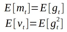
Now we need to correct the estimator, so that the expected value is the one we want. This step is usually referred to as bias correction. The final formulas for our estimator will be as follows:

The only thing left to do is to use those moving averages to scale learning rate individually for each parameter. The way it’s done in Adam is very simple, to perform weight update we do the following:

Advantages :
Adam converge faster than GD or SGD, in many settings. Especially for GANs, RL, and attention-based networks.
Adam might be able to converge to solutions with better quality (e.g. better local minima). This is based on my experience when playing with these algorithms for GANs and LSTM.
Disadvantages :
When Adam was first introduced, people got very excited about its power. Paper contained some very optimistic charts, showing huge performance gains in terms of speed of training:

Then, Nadam paper presented diagrams that showed even better results:

However, after a while people started noticing that despite superior training time, Adam in some areas does not converge to an optimal solution, so for some tasks (such as image classification on popular CIFAR datasets) state-of-the-art results are still only achieved by applying SGD with momentum. More than that Wilson et. al showed in their paper ‘The marginal value of adaptive gradient methods in machine learning’ that adaptive methods (such as Adam or Adadelta) do not generalize as well as SGD with momentum when tested on a diverse set of deep learning tasks, discouraging people to use popular optimization algorithms. A lot of research has been done since to analyze the poor generalization of Adam trying to get it to close the gap with SGD.
Nitish Shirish Keskar and Richard Socher in their paper ‘Improving Generalization Performance by Switching from Adam to SGD’ [5] also showed that by switching to SGD during training training they’ve been able to obtain better generalization power than when using Adam alone. They proposed a simple fix which uses a very simple idea. They’ve noticed that in earlier stages of training Adam still outperforms SGD but later the learning saturates. They proposed simple strategy which they called SWATS in which they start training deep neural network with Adam but then switch to SGD when certain criteria hits. They managed to achieve results comparable to SGD with momentum.
6. RMSProp optimization :
RMSprop is unpublished optimization algorithm designed for neural networks . RMSprop lies in the realm of adaptive learning rate methods, which have been growing in popularity in recent years, but also getting some criticism. It’s famous for not being published, yet being very well-known; most deep learning framework include the implementation of it out of the box.
There are two ways to introduce RMSprop. First, is to look at it as the adaptation of rprop algorithm for mini-batch learning. It was the initial motivation for developing this algorithm. Another way is to look at its similarities with Adagrad[2] and view RMSprop as a way to deal with its radically diminishing learning rates. I’ll try to hit both points so that it’s clearer why the algorithm works.
The RMSprop optimizer is similar to the gradient descent algorithm with momentum. The RMSprop optimizer restricts the oscillations in the vertical direction. Therefore, we can increase our learning rate and our algorithm could take larger steps in the horizontal direction converging faster. The difference between RMSprop and gradient descent is on how the gradients are calculated. The following equations show how the gradients are calculated for the RMSprop and gradient descent with momentum. The value of momentum is denoted by beta and is usually set to 0.9. If you are not interested in the math behind the optimizer, you can just skip the following equations.


Sometimes the value of v_dw could be really close to 0. Then, the value of our weights could blow up. To prevent the gradients from blowing up, we include a parameter epsilon in the denominator which is set to a small value.
disadvantages :
Learning rate is still manual, because the suggested value is not always appropriate for every task. Implementation of RMSProp Descent with Employee Attrition
7. Learning rate decay :

learning rate is a tuning parameter in an optimization algorithm that determines the step size at each iteration while moving toward a minimum of a loss function. Since it influences to what extent newly acquired information overrides old information, it metaphorically represents the speed at which a machine learning model “learns”. In the adaptive control literature, the learning rate is commonly referred to as gain.
In setting a learning rate, there is a trade-off between the rate of convergence and overshooting. While the descent direction is usually determined from the gradient of the loss function, the learning rate determines how big a step is taken in that direction. A too high learning rate will make the learning jump over minima but a too low learning rate will either take too long to converge or get stuck in an undesirable local minimum.
In order to achieve faster convergence, prevent oscillations and getting stuck in undesirable local minima the learning rate is often varied during training either in accordance to a learning rate schedule or by using an adaptive learning rate. The learning rate and its adjustments may also differ per parameter, in which case it is a diagonal matrix that can be interpreted as an approximation to the inverse of the Hessian matrix in Newton’s method.
The learning rate is related to the step length determined by inexact line search in quasi-Newton methods and related optimization algorithms.
The mathematical form of time-based decay is lr = lr0/(1+kt) where lr, k are hyperparameters and t is the iteration number. Looking into the source code of Keras, the SGD optimizer takes decay and lr arguments and update the learning rate by a decreasing factor in each epoch.
lr *= (1. / (1. + self.decay * self.iterations))References :
https://www.deepnetts.com/blog/from-basic-machine-learning-to-deep-learning-in-5-minutes.html
https://medium.com/greyatom/why-how-and-when-to-scale-your-features-4b30ab09db5e

